

Executive Summary 3
Data Understanding 4
Data Preparation 5
Dealing with Missing Value 5
Data Transformation & Feature Selection 6
Modeling 8
K-means Clustering 8
Visualising the distances between data points 10
First cluster plot with two centroids 10
Subsequent plots with more random centroids 11
Total within-clusters sum of squares 11
Elbow method 12
Average Silhouette Width 12
Gap Statistic 13
Results for k=4 Cluster Plot 13
Results for k=14 Cluster Plot 14
Mapped cluster numbers 16
Passenger profiles of major clusters 16
Recommendation for better customer experience 17
Logistic Regression 18
Split the data into training and testing set 18
Fitting a Logistic Regression model using training set 19
Confidence intervals of coefficient estimates 19
Exponentiate the coefficients and interpret them as odds-ratios 20
Prediction on test set with Logistic Regression 21
Compute Cross Table, Accuracy and Error Rate of Logistic Regression Model 22
Training Set Results 23
Testing Set Results 24
Logistic Regression Model Summary 25
Evaluation 27
Conclusion 28
References 42
Executive Summary
This report is based on the Titanic dataset from Kaggle with R Programming to apply necessary data understanding and preparation methods. The primary objective of this report is to build up an ML model to group Titanic passengers into similar groups to analyze the passengers’ profiles and provide recommendations on what could have been done to create a better customer experience; identify which independent variables in the dataset contribute most to the survival of passengers in the 1912 tragedy and determine if Logistic Regression is a better model to predict the probability of survival.
Cross-Industry Standard Process for Data Mining (CRISP-DM) methodology process is applied to this project as a framework for guidance that focuses on business issues and technical analysis. CRISP-DM put the data mining processes into six phases, as shown in Figure 1.

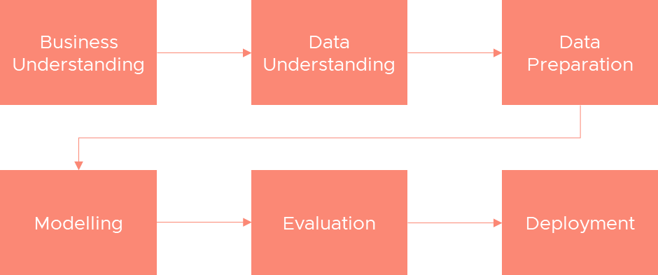
Figure 1 CRISP-DM Phases (“Data Mining using CRISP-DM methodology”, 2021)
Data Understanding
| Variable Name | Description | Var: Type | Value |
| PassengerID | Index number for the record | INT | Min – 1, Max – 1309 |
| Survived | Survival Status of the passenger | INT | 0= NO, 1=YES |
| Pclass | Ticket Class of the passenger | INT | 1= 1st class, 2= 2nd class, 3= 3rd class |
| Name | Passenger Name | CHR | |
| Sex | Gender of the passenger | CHR | |
| Age | Age of the passenger | NUM | Min – 0.17, Max – 80 |
| SibSp | No of Siblings/ Spouse onboard | INT | Min – 0, Max – 8 |
| Parch | No. of Parents/ Children onboard | INT | Min – 0, Max – 9 |
| Ticket | Ticket Number | CHR | |
| Fare | Ticket Fare | NUM | Min – 0, Max – 512.33 |
| Cabin | Cabin Number | CHR | |
| Embarked | Port of Embarkation | CHR | C = Cherbourg, Q = Queenstown, S = Southampton |
Table 1 List of variables with their descriptions
The Titanic Machine Learning dataset from Kaggle was used for this project to build a machine learning model using K-means Clustering and Logistic Regression techniques. The dataset included a total of 1,309 records with 12 attributes, as listed in Table 1.
Data Preparation
Dealing with Missing Value
| Variable Name | Missing Value |
| PassengerID | No Missing Value |
| Survived | No Missing Value |
| Pclass | No Missing Value |
| Name | No Missing Value |
| Sex | No Missing Value |
| Age | 263 Missing Values |
| SibSp | No Missing Value |
| Parch | No Missing Value |
| Ticket | No Missing Value |
| Fare | 1 Missing Value |
| Cabin | No Missing Value |
| Embarked | No Missing Value |
Table 2 List of variables with missing values
Table 2 shows which variable has a missing value in the selected dataset. The missing records will be excluded from the training dataset.
Remove all missing values
df2 <- na.omit(df)
df2 %>%
summarise_all(list(~is.na(.)))%>%
pivot_longer(everything(),
names_to = “variables”, values_to=”missing”) %>%
count(variables, missing) %>%
ggplot(aes(y=variables,x=n,fill=missing))+
geom_col()
list_missing <- colnames(df2)[apply(df2, 2, anyNA)]
list_missing


Figure 2 Screenshot of a chart generated to verify no missing values
Data Transformation & Feature Selection
We applied the data transformation method to “Sex” and “Embarked” variables as these two features were encoded as “CHR” originally. To include those two variables in the model building process, we transformed those two variables to “NUM”
| Variable Name | Original Var: Type | Target Var: Type | Value |
| Sex | CHR | NUM | 1= MALE, 0= FEMALE |
| Embarked | CHR | NUM | C= 12, Q= 26, S=28 |
Table 2 List of selected variables to be transformed

Figure 3 Screenshot of the dataset with Embarked and Sex variables transformed
As poor-quality data result in less accurate and unreliable performance results, we are removing the non-essential variables such as (i) PassengerID, (ii) Name, (iii) Ticket & (iv) Cabin from the model training dataset. Table 3 is the selected list of variables used in the model building process.
| Variable Name | Description | Var: Type | Value |
| Survived | Survival Status of the passenger | INT | 0= NO, 1=YES |
| Pclass | Ticket Class of the passenger | INT | 1= 1st class, 2= 2nd class, 3= 3rd class |
| Sex | Gender of the passenger | NUM | 1= MALE, 0= FEMALE |
| Age | Age of the passenger | NUM | Min – 0.17, Max – 80 |
| SibSp | No of Siblings/ Spouse onboard | INT | Min – 0, Max – 8 |
| Parch | No. of Parents/ Children onboard | INT | Min – 0, Max – 9 |
| Fare | Ticket Fare | NUM | Min – 0, Max – 512.33 |
| Embarked | Port of Embarkation | NUM | C= 12, Q= 26, S=28 |
Table 3 List of selected variables after Transformation & Filtering
Passenger ID, Name, Ticket, and Cabin variables were excluded as they are either nominal variables or unbalanced with too many missing values.

Figure 4 Screenshot of the transformed dataset with only selected features
Modeling
The model selection is a crucial stage for every Data Science project where the Data Scientist team has to decide on the appropriate algorithms which can provide the best result to meet their end goals. Generally, those algorithms can be classified into Supervised, Unsupervised, and Reinforcement Learning methods. For this project, we are choosing K-means Clustering to find the similarity in the passenger and Logistic Regression to predict the survivability of the passenger during the disaster.


Figure 5 Various Categories of Machine Learning Algorithms
K-means Clustering
K-means clustering is a Centroid-Based Clustering technique to classify the raw data into a number of groups, where k is a positive integer. Grouping of observation is based on calculating and minimizing the distance between the data points and their respect cluster centroid. The number of centroids depends on the number of required groups of clusters.

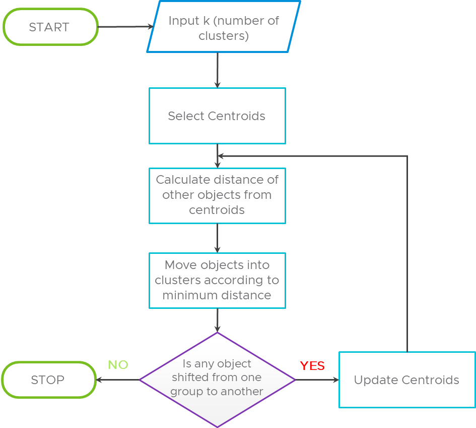
Figure 6 Flow Chart of K-Means Clustering Algorithm
The objective of K-means is to minimize the total distortion (within-cluster sum of squares WCSS), which is the sum of the distance of each observation in a cluster to its centroid.

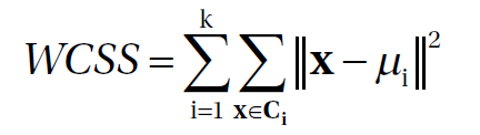
µi is the mean of the points in Ci
One of the vital steps of K-means clustering is choosing the optimal K value, which is more of an art than science. In practical application, an approximate K value is usually provided by the business. However, there are three popular methods to determine the optimal K values as follows:
1. Elbow Method
2. Sihouette Method
3. Gap statistics
Visualising the distances between data points

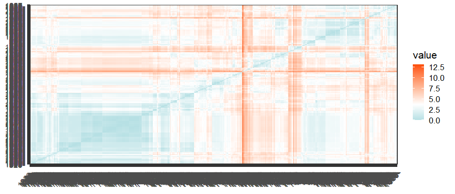
Figure 7 Distance Matrix to visualize the potential dissimilarities
From the output of functions get_dist and fviz_dist from the factoextra R package, the above heatmap illustrates passenger profiles with large dissimilarities (red) in contrast to those that appear to be similar.
First cluster plot with two centroids


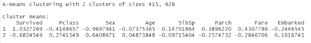
Figure 8 Results of k=2 clustering as an initial screening of data variances
Within cluster sum of squares by cluster:
[1] 3677.466 2864.141
(between_SS / total_SS = 21.5 %)
As seen in the above result, only approximately 21.5% of the total variance in this dataset is accountable by the two clusters formed.
Subsequent plots with more random centroids

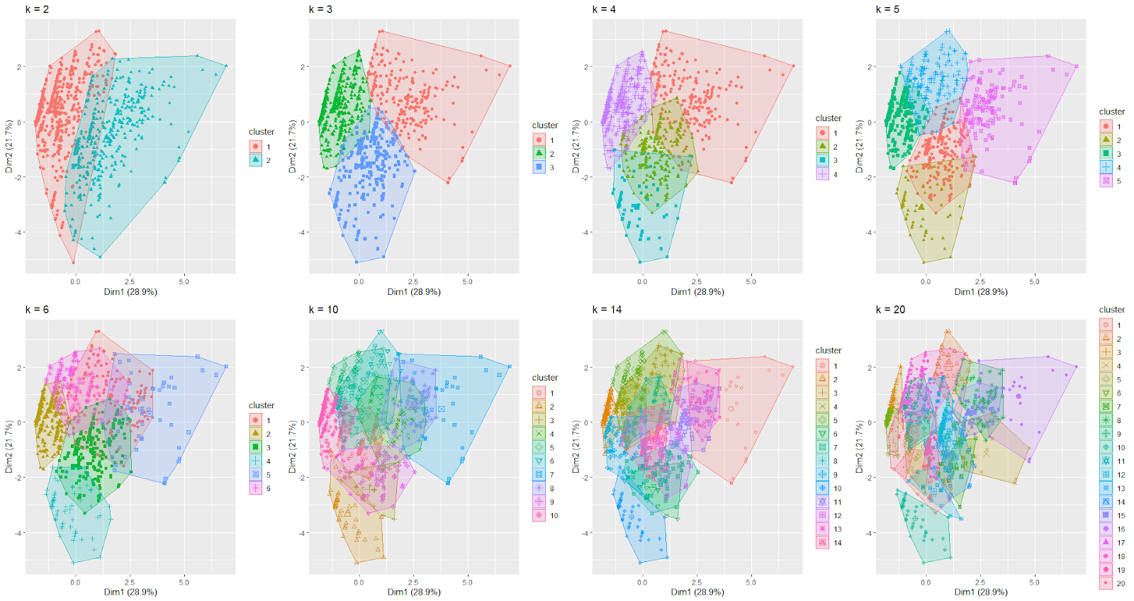
Figure 9 Visualisation of clusters with some random numbers of centroids
Since it is now known that two clusters were not sufficient to account for the groupings, a more random number of centroids were used to assess the optimal number of clusters.
The total within-clusters sum of squares
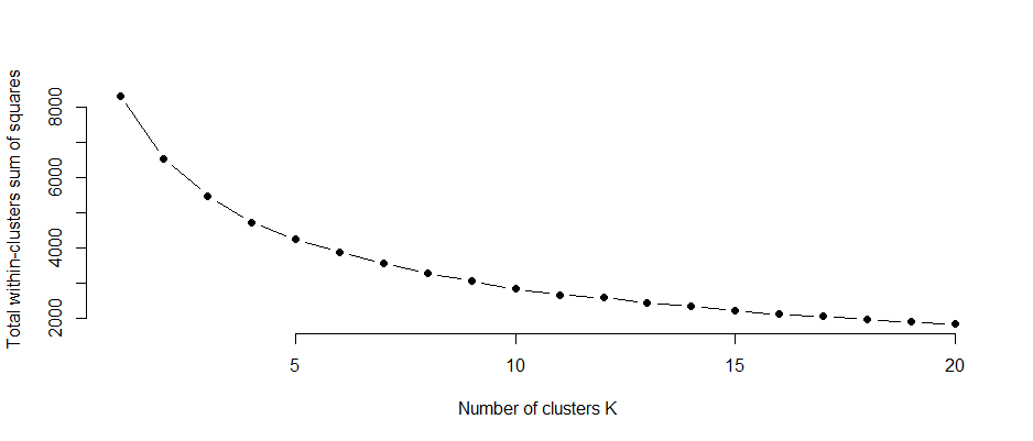
Figure 10 Chart showing the gradual reduction in the sum of squares as the number of clusters increased
Elbow method

Figure 11 Chart showing that k=4 or k=5 might be the optimal number of clusters based on the Elbow Method.
Average Silhouette Width

Figure 12 Chart showing that k=4 might be the optimal number of clusters based on the Average Silhouette Method since it produced the highest Average Silhouette Width between the clusters.
Gap Statistic
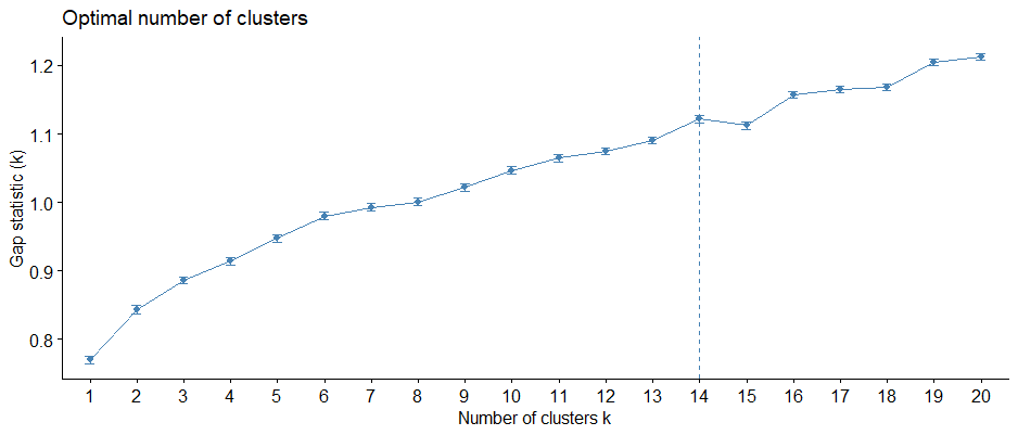
Figure 13 Gap Statistic chart showing k=14 as the optimal number of clusters, which means this clustering structure is the best grouping to assume no random uniform distribution of data points.
Based on the three methods presented above, k=4 and k=14 were identified as the optimal numbers of clusters. As such, Within Clusters Sum of Squares (WSS) for both k numbers was computed to determine the final clusters.
Results for k=4 Cluster Plot
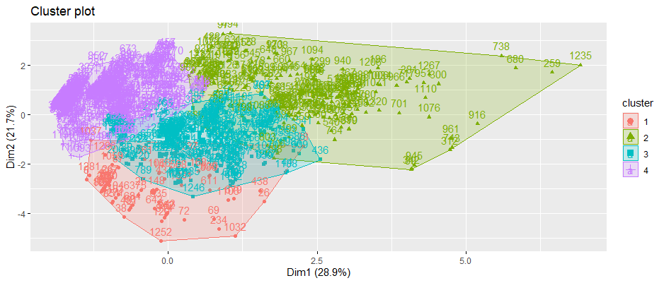
Figure 14 Visualization of 4 clusters

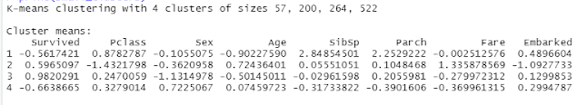
Figure 15 Results of k=4 clustering
Within cluster sum of squares by cluster:
[1] 498.1963 1675.3273 1133.6671 1419.7128
(between_SS / total_SS = 43.3 %)
Therefore, approximately 43.3% the total variance in this dataset is accountable by the four clusters formed.
Results for k=14 Cluster Plot
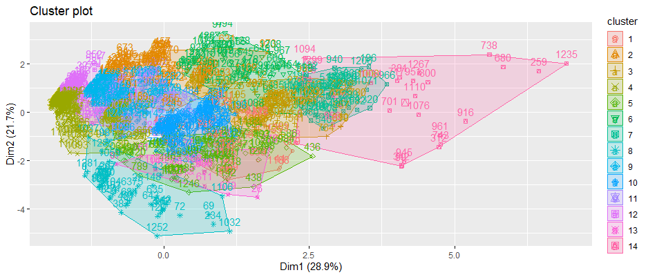
Figure 16 Visualization of k=14 clusters

Figure 17 Results of k=14 clustering
Within cluster sum of squares by cluster:
[1] 109.85184 171.84435 279.39369 303.61189 243.56093
[6] 172.22166 99.74677 144.01286 180.39667 144.61924
[11] 83.58127 94.80291 49.31257 277.18289
(between_SS / total_SS = 71.8 %)
Therefore, approximately 71.8% the total variance in this dataset is accountable by the fourteen clusters formed.
Based on the results above, k=14 was chosen to be the optimal number of clusters for further analysis.
Mapped cluster numbers

Figure 18 Screenshot of data frame with cluster numbers being assigned back to names of the passengers
Passenger profiles of major clusters
| Cluster No. | Size | Assessment of Passengers’ Profile |
| 4 | 227 | About 97.79% of the passengers embarked from Southhampton, about 10.13% are female about 9.25% of the passengers survived the majority Fare paid was about $7 to $9 |
| 9 | 127 | About 99.21% of the passengers embarked from Southhampton, about 2.36% are female about 3.14% of the passengers survive majority Fare paid was about $13 |
| 10 | 109 | About 91.74% of the passengers embarked from Southhampton, about 100% are female about 100% of the passengers survived the majority Fare paid was about $7 to $15 |
Table 4 Customers’ profiles within the major clusters computed
The larger clusters were chosen for further assessment of their inferred purchasing power and demographics.
Recommendation for better customer experience
Firstly, the major forms of entertainment on Titanic (“Onboard Titanic,” n.d.) were:
- Gambling
- Drinking
- Turkish Bath
- Gyms
- Shuffleboard
- Cricket
- Bull Board
- Tennis
- Chess
- Daily Sweepstakes
Since the majority of the passengers within the three clusters were male from Southhampton with a middle range of purchasing power inferred from the fare they paid, a targeted customer experience design revolving around this group of passengers could have enhanced the overall cruise experience.
In the context of the period when the Titanic set off in 1912, football was already a popular sport in England according to archives published on https://www.britishnewspaperarchive.co.uk/ . Therefore, the following top-performing football players from Southhampton F.C. during that era could have been invited to Titanic for a meet-and-greet as well as friendly matches on board the ship instead of having Cricket and Tennis as the sports entertainment. This would have likely boosted the demand for the Titanic experience even more.
Top scoring Southampton F.C. players from Year 1908 to 1912
| Player Name | Nationality | Pos | Club Career | Starting Appearances | Substitute Appearances | Total Appearances | Total Goals Scored |
| Arthur Hughes | FW | 1908–1909 | 28 | N/A | 28 | 18 | |
| Frank Jordan | FW | 1908–1910 | 56 | N/A | 56 | 10 | |
| Robert Carter | FW | 1909–1910 | 45 | N/A | 45 | 14 | |
| Charlie McGibbon | FW | 1909–1910 | 32 | N/A | 32 | 24 |

Table 5 Source: (“List of Southampton F.C. players (25–99 appearances),” 2012)
Logistic Regression
A regression model with a categorical target variable, attaining only two possible values (0 and 1) is known as Logistic regression. To model binary dependent variables, LR employs a logistic/ sigmoid function.
Logistic regression can be subdivided into three types based on the type of response variable:
1. Binomial Logistic Regression – Only two possible values for target variables
2. Multinomial Logistic Regression – Three or more values, but no fixed order of preference.
3. Ordinal Logistic Regression – Three or more possible values, each of which has a preference or order
Split the data into training and testing set
# split into training (80%) and testing set (20%)
sample_size = round(nrow(df7)*.80)
index <- sample(seq_len(nrow(df7)), size = sample_size)
train_set <- df7[index, ]
test_set <- df7[-index, ]
train_label <- train_set$Survived
test_label <- test_set$Survived
The above R code was used to divide the dataset into 80% training and 20% testing data.
Fitting a Logistic Regression model using the training set

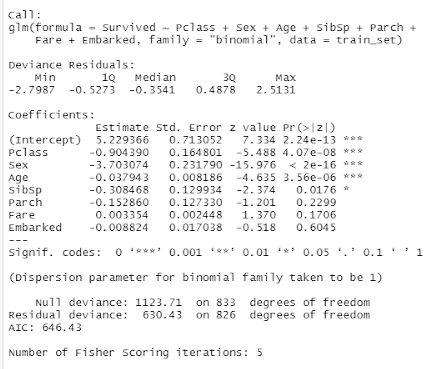
Figure 18 Screenshot of the Logistic Regression Model fitted using training set
The coefficients accounts for the change in the outcome in log odds for every one unit of increase of the predictors variable. The table showed that PClass, Sex and Age variables were all statistically significant.
Confidence intervals of coefficient estimates

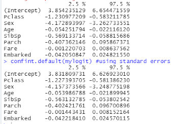
Figure 19 Screenshot of the computed confidence intervals
> # Test the overall effect of the PClass, Sex and Age as independent variables
> wald.test(b = coef(mylogit), Sigma = vcov(mylogit), Terms = 2:4)
Wald test:
———-
Chi-squared test:
X2 = 258.7, df = 3, P(> X2) = 0.0
The Wald Test results proved that since the chi-squared test statistic of 258.7 with 3 degrees of freedom has a p-value of 0.0, the difference between the coefficients of PClass, Sex and Age is statistically significant.
Exponentiate the coefficients and interpret them as odds-ratios

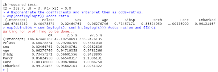
Figure 20 Screenshot of the computed odds ration binded to the coefficients intervals
When the coefficients were exponentiated, the odds-ratios showed that Fare does not the affect the odds of Survived. In contrast, it appears that Sex odds-ratio means the probability of male’s survival chance was very low.
Prediction on training set with Logistic Regression
# Create prediction for passengers’ survival on training set
train_set$SurvivedP <- predict(mylogit, newdata = train_set, type = “response”)
train_set
df8 <- cbind(train_set, predict(mylogit, newdata = train_set, type = “link”,
se = TRUE))
df8 <- within(df8, {
PredictedProb <- plogis(fit)
LL <- plogis(fit – (1.96 * se.fit))
UL <- plogis(fit + (1.96 * se.fit))
})

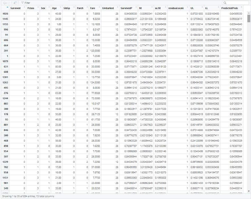
Figure 22 Screenshot of prediction done on training set for result comparison purpose
Prediction on test set with Logistic Regression
# Create a prediction on test set
test_set$SurvivedP <- predict(mylogit, newdata = test_set, type = “response”)
test_set$SurvivedP
df20 <- cbind(test_set, predict(mylogit, newdata = test_set, type = “link”,
se = TRUE))
df20 <- within(df20, {
PredictedProbTest <- plogis(fit)
LL <- plogis(fit – (1.96 * se.fit))
UL <- plogis(fit + (1.96 * se.fit))
})

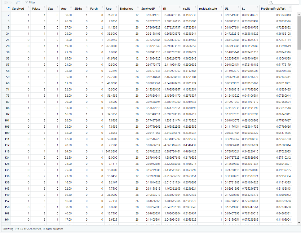
Figure 23 Screenshot of prediction done on test set for result comparison purpose
Compute Cross Table, Accuracy and Error Rate of Logistic Regression Model
Due to the incompatible versions of the R packages, library and Studio associated with Confusion Matrix, the originally intended code was not executable:
# Create Confusion Matrix
Cmatrix <- confusionMatrix(data=prediction_test, reference = df7$Survived)
Therefore, the following computation and calculation were made in lieu of the above issue:
Training Set Results

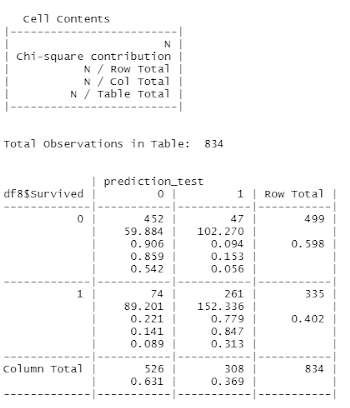
Figure 24 Screenshot of crosstable calculations
Accuracy = (TN + TP) / (TN + FN + FP + TP)
= (452 + 261) / (452 + 74 + 47 + 261)
= 0.854916
Therefore, the Accuracy of training set is approximately 85%.
Error Rate = (FN + FP) / (TN + FN + FP + TP)
= (74 + 47) / (452 + 74 + 47 + 261)
= 0.145084
Therefore, the Error Rate of training set is approximately 15%
Testing Set Results

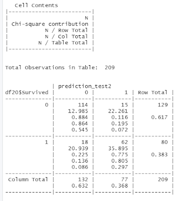
Figure 24 Screenshot of prediction done on test set for result comparison purpose
Logistic Regression Accuracy = (TN + TP) / (TN + FN + FP + TP)
= (114 + 62) / (114 + 18 + 15 + 62)
= 0.842105
Therefore, the Accuracy of test set prediction is approximately 84%.
Logistic Regression Error Rate = (FN + FP) / (TN + FN + FP + TP)
= (18 + 15) / (114 + 18 + 15 + 62)
= 0.157895
Therefore, the Error Rate of test set prediction is approximately 16%
Logistic Regression Model Summary
Since
> with(mylogit, null.deviance – deviance)
[1] 493.2767
> with(mylogit, df.null – df.residual)
[1] 7
> with(mylogit, pchisq(null.deviance – deviance, df.null – df.residual, lower.tail = FALSE))
[1] 2.235123e-102
> logLik(mylogit)
‘log Lik.’ -315.2161 (df=8)
Therefore, the chi-square of 493.2767 with 7 degrees of freedom, p-value of less than 0.001 suggests that the model generally fits significantly better than an empty model.
Conclusion
- K-means clustering and Logistic Regression were successfully applied to model the Titanic dataset.
- k=4 and k=14 were identified as the optimal number of clusters to group the Titanic passengers based on Gap Statistics, Elbow, and Average Silhouette Width methods.
- 3 major clusters of passengers were identified and recommendation for better customer experience was made more this customer segment.
- Logistic Regression was applied to determine that PClass, Sex, and Age variables’ effect on the Survival were statistically significant. The fitted model took 5 Fisher Score iterations to achieve approximately 84% accuracy in the prediction of passengers’ survival.
What the models could possibly do is predict the probability of survival of a person from our times, if he were born in the late 19th century and went on board the Titanic ship in 1912 as a teenager from Queenstown. Likewise for the k-means clusters generated, profiles of the groups would only be as good as the context which the features could help the researcher to interpret. The key takeaway from this study was that this clustering technique could be applied to other passengers on other ships and routes beforehand to provide meaningful information for the service provider to act on. This market intelligence could help marketing and operational functions craft better itineraries and make better logistic arrangements that are customer-focused with a design thinking approach.
References
Data mining using CRISP-DM methodology. (n.d.). Engineering Education (EngEd) Program | Section. https://www.section.io/engineering-education/data-mining-using-crisp-dm-methodology/
List of Southampton F.C. players (25–99 appearances). (2012, November 15). Wikipedia, the free encyclopedia. Retrieved November 25, 2021, from https://en.wikipedia.org/wiki/List_of_Southampton_F.C._players_(25%E2%80%9399_appearances)On board Titanic. (n.d.). The History Press | The destination for history. https://www.thehistorypress.co.uk/titanic/on-board-titanic/